モデルの確認
本検定のためのモデルについてはこちらの姉妹記事で詳細を説明していますので、ここでは要点だけ記載しておくことにします。
このとき、我々の興味の対象となる確率変数は
これらは、従来の仮説検定における片側検定・両側検定に対応します。
Unrestricted Model
では、
まずはサンプルデータを準備します。
# sample data

#x1:Group1
x1 <- c(rbinom(n=40, size=1, prob=0.4),rbinom(n=60, size=1, prob=0.5))
#x2:Group2
x2 <- c(rbinom(n=40, size=1, prob=0.2),rbinom(n=60, size=1, prob=0.5))

library(ggplot2)
library(gridExtra)

p1 <- ggplot(data=data.frame(X=x1)) + theme_light(base_size=11) + geom_bar(aes(x=X), fill="#004C98") +
  scale_x_continuous(breaks=c(0,1), labels = c("-","危険挙動")) + xlab("Group1")
p2 <- ggplot(data=data.frame(X=x2)) + theme_light(base_size=11) + geom_bar(aes(x=X), fill="#004C98") +
  scale_x_continuous(breaks=c(0,1), labels = c("-","危険挙動")) + xlab("Group2")

p <- grid.arrange(p1, p2, ncol=2)
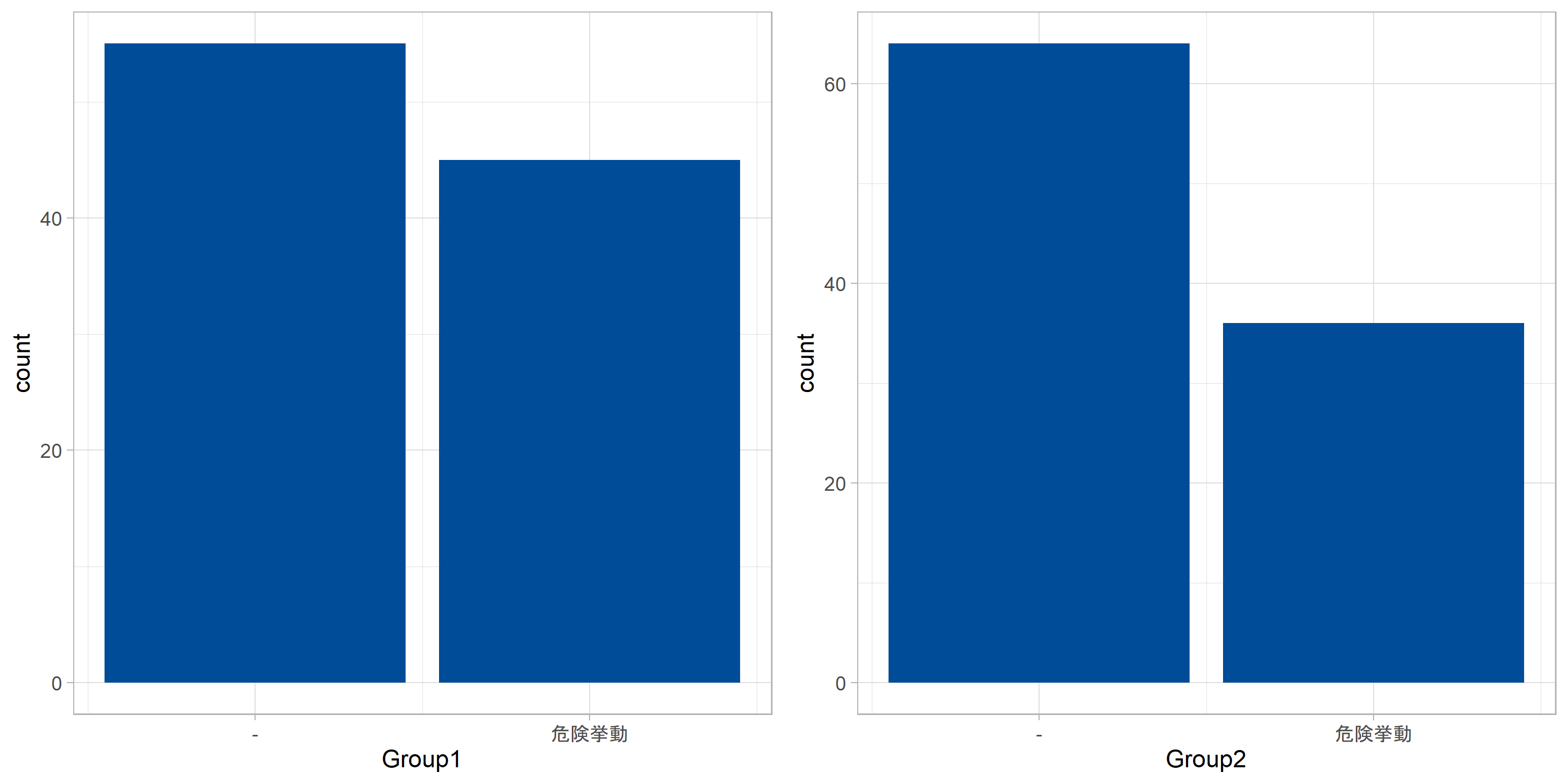
このデータに対し、通常の比率の差の検定を関数prop.test()で行います。原理は昔紹介した分割表の一様性の検定と同じものです。
prop.test(x=c(sum(x1),sum(x2)), n=c(length(x1),length(x2)), correct=F)

## 2-sample test for equality of proportions without continuity correction
##
## data:  c(sum(x1), sum(x2)) out of c(length(x1), length(x2))
## X-squared = 1.6807, df = 1, p-value = 0.1948
## alternative hypothesis: two.sided
## 95 percent confidence interval:
## -0.04549292  0.22549292
## sample estimates:
## 0.45   0.36
## prop 1 prop 2
2グループの比率が同じであるという帰無仮説を設定した検定に対し、p値
次にこちらの記事の
data <- list(N1=length(x1), N2=length(x2), S1=sum(x1), S2=sum(x2))

# calculate BF_01 by closed form
# data[[1]]:n1
# data[[2]]:n2
# data[[3]]:s1
# data[[4]]:s2

cat(choose(data[[1]],data[[3]]) * choose(data[[2]],data[[4]]) / choose(data[[1]]+data[[2]], data[[3]]+data[[4]])*(data[[1]]+1)*(data[[2]]+1)/(data[[1]]+data[[2]]+1))

## 2.526656
対立仮説
以上、検定結果をひととおり見た上で、次はMCMCにより
//non-restricted aalysis
//model1.stan
data {
  //the number fo sample of Group1
  int<lower=1> N1;
  //the number fo sample of Group2
  int<lower=1> N2;
  //the number fo sample which occurs with a probability of theta1 of Group1
  int<lower=0> S1;
  //the number fo sample which occurs with a probability of theta2 of Group2
  int<lower=0> S2;
}


parameters {
  //the parameter of Binomial distribution of Group1
  real<lower=0, upper =1> theta1;
  //the parameter of Binomial distribution of Group2
  real<lower=0, upper=1> theta2;
}

model {
  //S1 ~ binomial(N1, theta1)
  target += binomial_lpmf(S1 | N1, theta1);
  //S2 ~ binomial(N2, theta2)
  target += binomial_lpmf(S2 | N2, theta2);

  //uninformative prior
  target += beta_lpdf(theta1 | 1,1);
  target += beta_lpdf(theta2 | 1,1);
}

generated quantities{
  //the difference parameter between theta1 and theta2
  real delta;
  delta = theta1 - theta2;
}
iterationを
options(mc.cores = parallel::detectCores())
rstan_options(auto_write = TRUE)
fit <- stan(file="model/model1.stan", data=data, iter=11000, warmup=1000, chain=4)
fit

## Inference for Stan model: model1.
## 4 chains, each with iter=11000; warmup=1000; thin=1;
## post-warmup draws per chain=10000, total post-warmup draws=40000.
##
##         mean se_mean   sd   2.5%   25%   50%   75% 97.5% n_eff Rhat
## theta1  0.45    0.00 0.05   0.36  0.42  0.45  0.48  0.55 36883    1
## theta2  0.36    0.00 0.05   0.27  0.33  0.36  0.39  0.46 36917    1
## delta   0.09    0.00 0.07  -0.05  0.04  0.09  0.13  0.22 36034    1
## lp__   -8.89    0.01 1.02 -11.60 -9.27 -8.58 -8.17 -7.90 17925    1
このシミュレーション結果を使って
library(ggplot2)
library(ggrepel)
library(logspline)
library(tidyverse)

# non_restricted analysis
d <- as.matrix(fit)[,"delta"]
fit_logspline <- logspline(d)

plot_title = ggtitle(label="equalty of proportions(unrestricted analysis)")
p <- ggplot() + theme_light(base_size=11) +
  geom_path(data=data.frame(X=x <- seq(-1,1,0.01), Y=dlogspline(x,fit_logspline)), aes(x=X,y=Y), color="blue") +
  geom_line(data=data.frame(x=c(-1,0,1),y=c(0,1,0)),aes(x=x,y=y)) +
  geom_point(data=data.frame(x=0,y=dlogspline(0, fit_logspline)),aes(x=x,y=y), color="blue") +
  geom_point(data=data.frame(x=0,y=1), aes(x=x, y=y)) +
  geom_text_repel(data=data.frame(x=c(0,0),y=c(1,dlogspline(0,fit_logspline)),label=c(1,round(dlogspline(0, fit_logspline),2))),
                  aes(x=x,y=y,label=label)) +
  annotate("text",x=-Inf,y=Inf,label=sprintf("BF01=%.2f",dlogspline(0,fit_logspline)),hjust=-.2,vjust=2) + plot_title
p
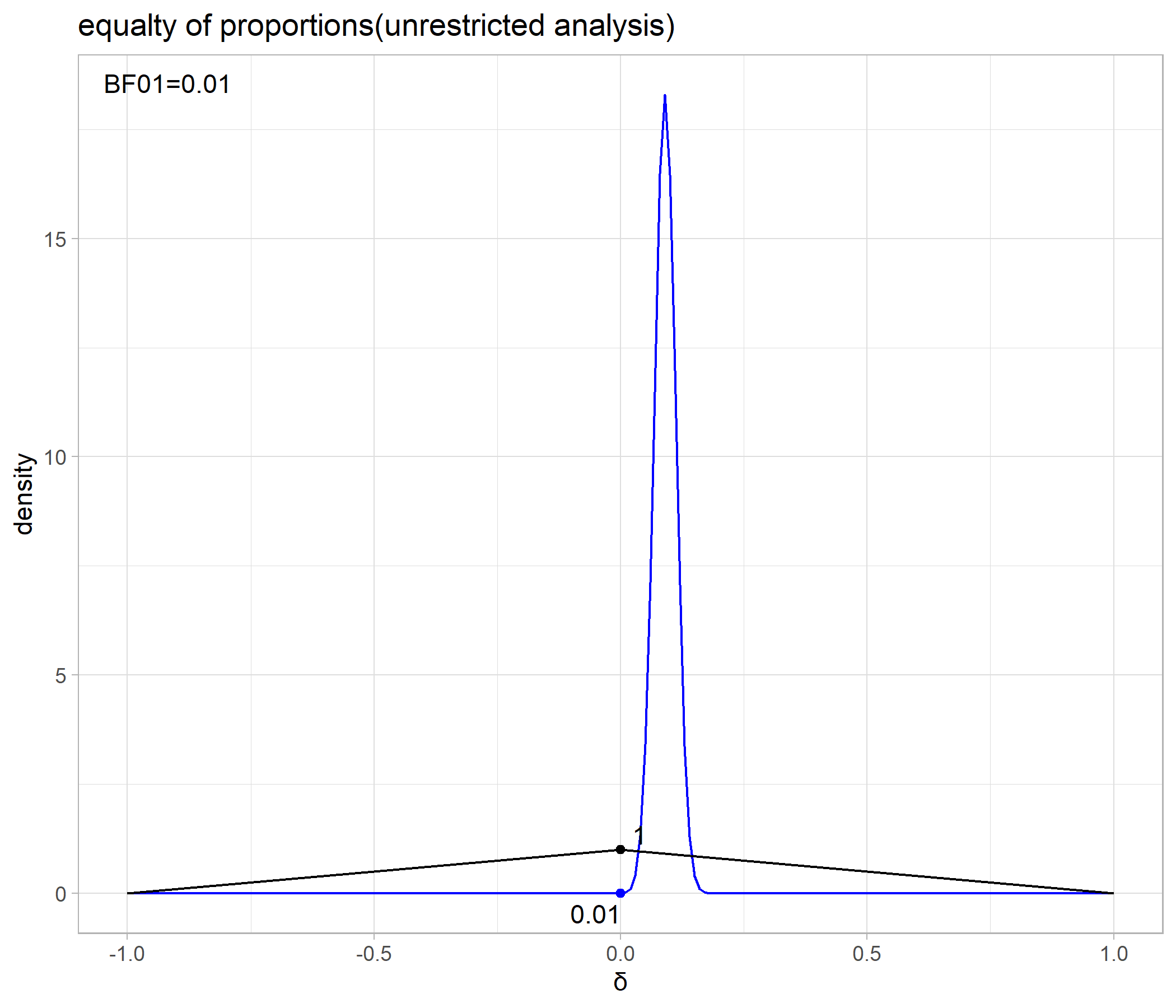
結果は、
同じ危険挙動発生率でも標本数が倍になると、確信をもって差があると言える程度も変わってくるはずです。ちょっと確認してみましょう。
# data with same probability but twice sample size
#new_x1:Group1
new_x1 <- rep(x1,10)
#new_x2:Group2
new_x2 <- rep(x2,10)

~(以下略)~

cat(1/dlogspline(0,fit_logspline))
## 147.1852
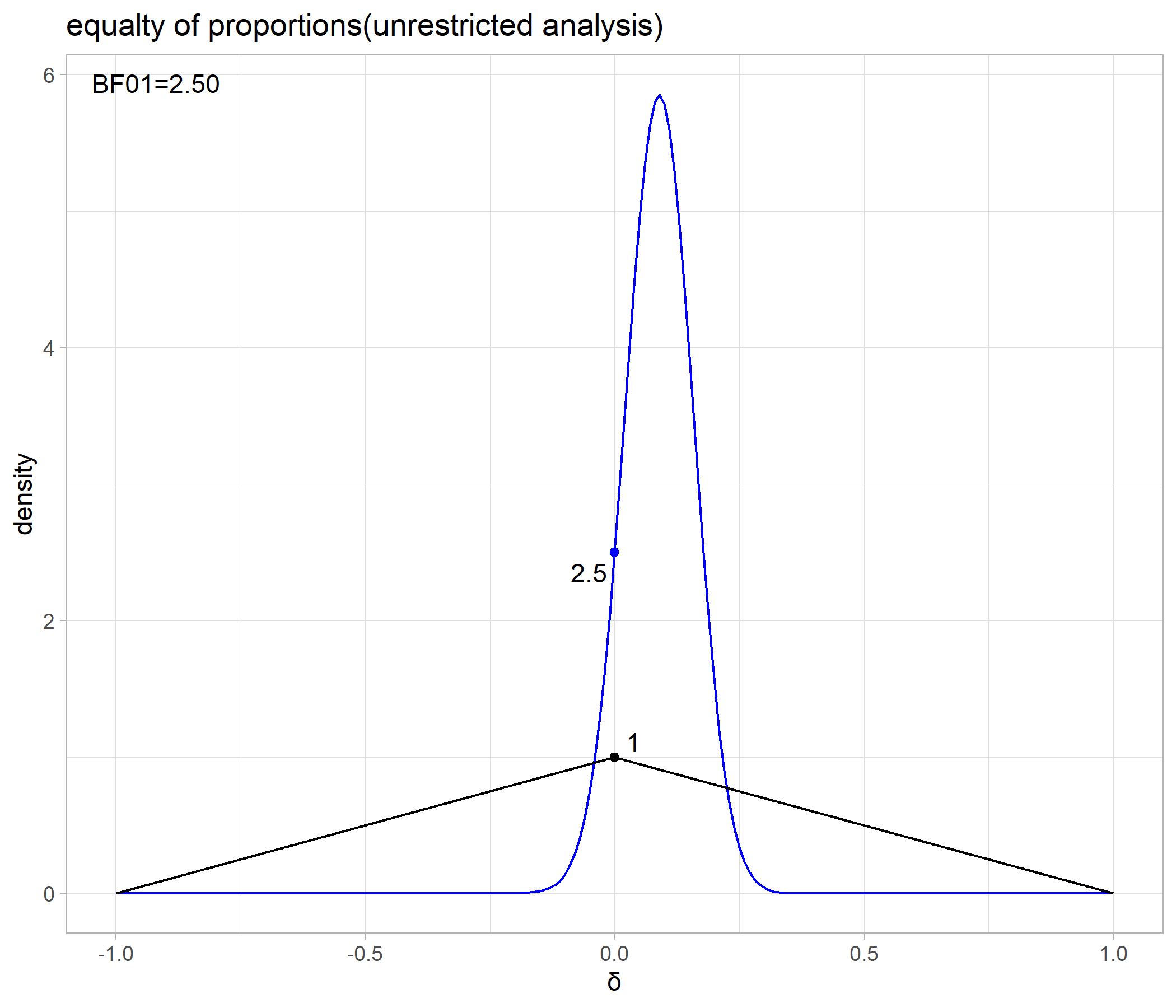
Order-restricted Model
次に、
# restricted analysis
fit_logspline <- logspline(d)

dens <- function(x){
  dlogspline(x, fit_logspline)/(1-plogspline(0, fit_logspline))}

plot_title = ggtitle(label="equalty of proportions(order-restricted analysis)")
p <- ggplot() + theme_light(base_size=11) +
  geom_path(data=data.frame(X=x <- seq(0,1,0.001), Y=dens(x)), aes(x=X,y=Y), color="blue") +
  geom_line(data=data.frame(x=c(0,1),y=c(2,0)),aes(x=x,y=y)) +
  geom_point(data=data.frame(x=0,y=dens(0)),aes(x=x,y=y), color="blue") +
  geom_point(data=data.frame(x=0,y=2), aes(x=x, y=y)) +
  geom_text_repel(data=data.frame(x=c(0,0),y=c(2,dens(0)),label=c(2,round(dens(0),2))),
                  aes(x=x,y=y,label=label)) +
  annotate("text",x=Inf,y=Inf,label=sprintf("BF01=%.2f",dens(0)/2),hjust=1.2,vjust=2) +
  xlab("δ") + ylab("density") + plot_title
p

cat(dens(0)/2)
## 1.385902
検定の結果は、Unrestricted Modelが
またベイズファクターは相対比較ですから、
よって、
ここまで、対応の無い比率のさの検定をベイズファクターを使って実践してみました。従来通りの結果と比べて理論が簡潔で私は好みのベイズファクター、「分かりやすい」統計のために今後重要になってくるのではないでしょうか。
一方、本例のような危険挙動データの例の場合、本来、危険挙動を観測した車両の全体に占める割合は非常に小さく、通常1割にも達しません(私の経験)。
このようなデータに対し、二項分布のパラメータ
おわりに
今回は、ベイズファクターを使って比率の差を検定する方法を実践しました。解析的に求める方法と、MCMCを使って近似的に求める方法の2通りを実践しましたが、精度の面からいうともちろん解析的に求めるのが妥当です。しかし、後半で実践したような、Order-restricted Modelで検定したいときなどは、解析解をまた別に求めてやらなばなりません。こちらの記事で導出した解析解はあくまで従来通りの検定における帰無仮説と対立仮説の(方向性をもたない)比較をしたいときの解であり、この式だけでは他の仮説の比較に応用できないのです。それならOrder-restricted Modelの解析解を求めてやれば良いのですが、目的に応じてその都度解を求めるのは大変です。MCMC法はそういった面倒な計算をすっ飛ばして近似的にベイズファクターやら事後分布やらを求めることができる、という点が魅力的なんですね(といっても今回は片側検定に対応するモデルしかMCMC法で追加検討していませんが)。